Cucurbitales platform

Software tutorial

Blast

Reference: Basic local alignment search tool

Download: ncbi-blast-2.13.0+-x64-linux.tar.gz ↗ [Source]

wget ftp://ftp.ncbi.nlm.nih.gov/blast/executables/blast+/LATEST/ncbi-blast-2.13.0+-x64-linux.tar.gz

Installation:

#Unzip
tar -zxvf ncbi-blast-2.13.0+-x64-linux.tar.gz
#Rename
mv ncbi-blast-2.13.0+-x64-linux blast
#Environment variable settings
Edit the ~/.bashrc file and add the following line at the end:
export PATH=/home/local/Software/blast/bin:$PATH
#Configuration effective
source ~/.bashrc

Use Flow:

# Makeblastdb:
makeblastdb -in db.fasta -dbtype prot -parse_seqids -out dbname(format database)
# Parameter description:
-in: the sequence file to be formatted
-dbtype: database type, prot or nucl
-out: database name
-parse_seqids: parse sequence identifier (recommended to add)
# Blastp:
blastp -query seq.fasta -out seq.blast -db dbname -outfmt 6 -evalue 1e-5 -num_descriptions 10 -num_threads 8 (protein sequence comparison protein database)
# Blastn:
blastn -query seq.fasta -out seq.blast -db dbname -outfmt 6 -evalue 1e-5 -num_descriptions 10 -num_threads 8 (nucleic acid sequence comparison nucleic acid database)
# Blatsx:
blastx -query seq.fasta -out seq.blast -db dbname -outfmt 6 -evalue 1e-5 -num_descriptions 10 -num_threads 8 (nucleic acid sequence comparison protein database)
# Parameter Description:
-query: input file path and file name
-out: output file path and file name
-db: formatted database path and database name
-outfmt: output file format, there are 12 formats in total, 6 are tabular format corresponding to BLAST's m8 format
-evalue: set the e-value value of the output result
-num_descriptions: the number of output results in tabular format
-num_threads: number of threads
-max_target_seqs 5: output the result of up to 5 comparisons, if it is 1, it is the best match
## Above is the comparison result of blast, there are 12 columns, which represent.
1, Query id: query sequence ID identification (blast comparison sequence)
2、Subject id: the ID of the target sequence on the comparison (library building sequence)
3、identity: the consistency percentage of sequence matching
4、alignment length: the length of the alignment area that matches the comparison
5、mismatches: the number of mismatches in the alignment area
6、gap openings: the number of gaps in the matching region
7, start: the starting position of the matching region on the query sequence (Query id)
8, end: the end point of the comparison region on the query id
9, start: the start of the comparison region in the target sequence (Subject id)
10, end: the end point of the comparison region in the target sequence (Subject id)
11, e-value: the expected value of the comparison result
12、bit score: the bit score value of the comparison result
In general, we look at columns 3, 11 and 12, the smaller the e-value, the more reliable.

Notice:

# When comparing the makeblastdb library with blast, pay attention to the parameters, whether the protein file is used or the nucleic acid file.

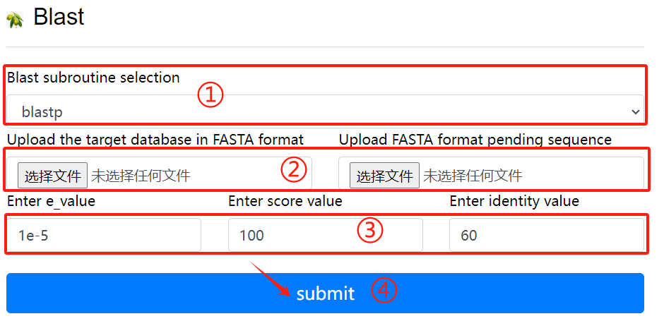
Blast usage:

1. Select the desired blast subroutine
2. Submit fasta format files respectively
   to form library files and files that
   need to be compared
3. Select the required parameters
4. Click the submit button

Diamond

Reference: Fast and sensitive protein alignment using DIAMOND

Download: diamond-linux64.tar.gz ↗ [Source]

Installation:

#Unzip
tar zxf diamond-linux64.tar.gz
#Rename
mv diamond ~/bin
#Environment variable settings
echo 'PATH=$PATH:/root/bin' >> ~/.bashrc
#Configuration effective
source ~/.bashrc

Use Flow:

## linux command:
# Build a database
    diamond makedb --in nr --db nr
## Sequence alignment
# Nucleic acid
    diamond blastx --db nr -q reads.fna -o dna_matches_fmt6.txt
# Protein
    diamond blastp --db nr -q reads.faa -o protein_matches_fmt6.txt

Notice:

# When comparing the diamond makedb library with diamond blast, pay attention to the parameters, whether the protein file is used or the nucleic acid file.

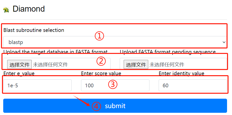
Diamond usage:

1. Select the desired blast subroutine
2. Submit fasta format files respectively
   to form library files and files that
   need to be compared
3. Select the required parameters
4. Click the submit button

MCScanX

Reference: MCScanX: a toolkit for detection and evolutionary analysis of gene synteny and collinearity

Download: MCScanX-master.zip ↗ [Source]

Installation:

#Unzip:
unzip MCScanX-master.zip
#Compile
make

Use Flow:

## Before running MCScanX, we need to put the gff file, blast file into the same folder and the gff file is the gff of two species gff files merged. the other two files need to have the same name.
    MCScanX se_so
# Plotting covariance points
    java dot_plotter -g se_so.gff -s se_so.collinearity -c dot.ctl -o dot.PNG

Common error sets:

#   error 1: “msa.cc:289:9: error: ‘chdir’ was not declared in this scope”
    solve 1: open "msa.cc", add #include <unistd.h> at the top

#   error 2: “dissect_multiple_alignment.cc:252:44: error: ‘getopt’ was not declared in this scope”
    solve 2: open "dissect_multiple_alignment.cc", add #include <getopt.h> at the top

#   error 3: “detect_collinear_tandem_arrays.cc:286:17: error: ‘getopt’ was not declared in this scope”
    solve 3: open "detect_collinear_tandem_arrays.cc", add #include <getopt.h> at the top

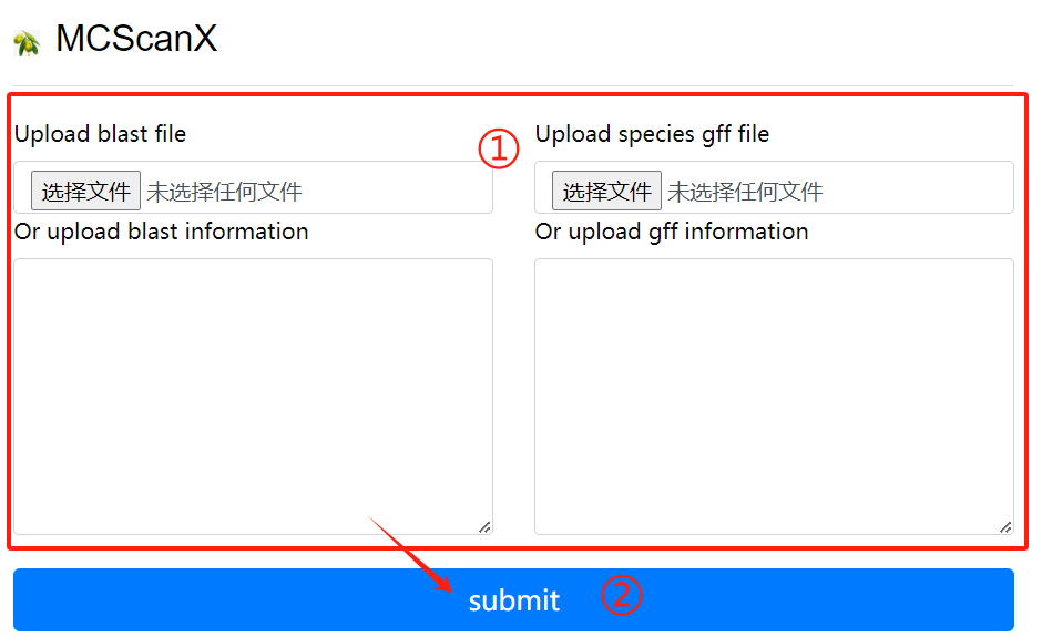
MCScanX usage:

1. Upload or enter the blast file and the
   corresponding gff file in the input
   field
2. Click the submit button

Colinearscan

Reference: Statistical inference of chromosomal homology based on gene colinearity and applications to Arabidopsis and rice

Download: ↗ [Source]

Use Flow:

# Extracting gene pairs from BLAST results
    cat ath_chr2_indica_chr5.blast | get_pairs.pl --score 100 > ath_chr2_indica_chr5.pairs
# Masking of highly repetitive loci
    cat ath_chr2_indica_chr5.pairs | repeat_mask.pl -n 5 > ath_chr2_indica_chr5.purged
# Estimate maximum gap length
    max_gap.pl --lenfile ath_chrs.lens --lenfile indica_chrs.lens --suffix purged
# Detect covariate fragments
    block_scan.pl --mg 321000 --mg 507000 --lenfile ath_chrs.lens --lenfile indica_chrs.lens --suffix purged
## For efficiency, the above process can also be written as a shell script with the following code.

    #!/bin/sh
    do_error()
    {
     echo "Error occured when running $1"
     exit 1
    }
    
    echo "Start to run the working example..."
    echo
    
    echo "* STEP1 Extract pairs from BLAST results"
    echo "  We should parse BLAST results and extract pairs of anchors (genes in this example) satisfying our rule (score >= 100)."
    echo
    echo "  > cat ath_chr2_indica_chr5.blast | get_pairs.pl --score 100 > ath_chr2_indica_chr5.pairs"
    echo
    cat ath_chr2_indica_chr5.blast | get_pairs.pl --score 100 > ath_chr2_indica_chr5.pairs || do_error get_pairs.pl
    echo
    
    echo "* STEP2 Mask highly repeated anchor"
    echo "  Highly repeated anchors which are mostly generated by continuous single gene duplication events make those colinear segements vague to be detected. We mask them off using a very simple algorithm."
    echo
    echo "  > cat ath_chr2_indica_chr5.pairs | repeat_mask.pl -n 5 > ath_chr2_indica_chr5.purged"
    echo
    cat ath_chr2_indica_chr5.pairs | repeat_mask.pl -n 5 > ath_chr2_indica_chr5.purged || do_error repeat_mask.pl
    echo
    
    echo "* STEP3 Estimate maximum gap length"
    echo "  Use pair files with repeats masked to estimate mg values which will be used to detected colinear blocks."
    echo
    echo "  > max_gap.pl --lenfile ath_chrs.lens --lenfile indica_chrs.lens --suffix purged"
    echo
    max_gap.pl --lenfile ath_chrs.lens --lenfile indica_chrs.lens --suffix purged || do_error max_gap.pl
    echo
    
    echo "* SETP4 Detect blocks from pair file(s)"
    echo "  Everything's ready do scan at last."
    echo
    echo "  > block_scan.pl --mg 321000 --mg 507000 --lenfile ath_chrs.lens --lenfile indica_chrs.lens --suffix purged"
    echo
    block_scan.pl --mg 321000 --mg 507000 --lenfile ath_chrs.lens --lenfile indica_chrs.lens --suffix purged || do_error block_scan.pl
    echo
    
    echo "Now ath_chr2_indica_chr5.blocks contains predicted colinear blocks."

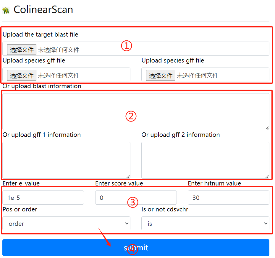
Colinearscan usage:

1. Upload the target blast file and the gff
   file corresponding to the two genomes
2. Or enter the target blast file, the
   corresponding two gff files, in the
   input field
3. Select the required parameters
4. Click the submit button

ParaAT

Reference: ParaAT: A parallel tool for constructing multiple protein-coding DNA alignments, Biochem Biophys Res Commun

Download: ParaAT2.0.tar.gz ↗ [Source]

ParaAT2.0 download address is: https://ngdc.cncb.ac.cn/tools/paraat

Use Flow:

# "ParaAT.pl" is the running script, you can use it directly after downloading and unpacking. You can add the unpacked path to the environment variable or use the absolute path where the script is located to run it.
# Dependency Tools Download
# 1. Protein comparison tools: such as clustalw2, mafft, muscle, etc.
# 2. Kaks_Calculator (https://ngdc.cncb.ac.cn/tools/kaks)
Run ParaAT
    ParaAT.pl -h test.homologs -n test.cds -a test.pep -p proc -m muscle -f axt -g -k -o result_dir

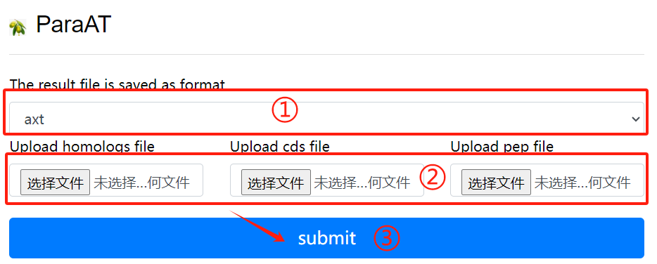
ParaAT usage:

1. Select result of the need to save the
   file format
2. Upload the required homologs file
   cds file and pep file
3. Select the required parameters
4. Click the submit button

KaKs_Calculator

Reference: KaKs_Calculator 3.0: Calculating Selective Pressure on Coding and Non-coding Sequences

Download: KaKs_Calculator3.0.zip ↗ [Source]

KaKs_Calculator3 download address is: https://ngdc.cncb.ac.cn/biocode/tools/BT000001

Installation:

unzip KaKs_Calculator3.0.zip
# Compile KaKs
cd KaKs_Calculator3.0 && make
# Main programs: KaKs, KnKs, AXTConvertor
# Unzip and add environment variables
Install ParaAT, the installation method can be seen in Hear.

Use Flow:

# Prepare input files
    test.cds # DNA sequence of each gene
    test.pep #Protein sequences for each gene
    The proc file contains a number indicating the number of CPU calls
# Start analysis
    ParaAT.pl -h test.homolog -n test.cds -a test.pep -p proc -m mafft -f axt -g -k -o result_dir
# ParaAT.pl parameters explained.
     -h, homologous gene name file
     -n, file of specified nucleic acid sequences
     -a, specified protein sequence file
     -p, specifies the multithreaded file numbers
     -m, specifies the comparison tool (clustalw2 | t_coffee | mafft | muscle), multiple choice
     -g, remove codons with gaps
     -k, use KaKs_Calculator to calculate kaks values
     -o, output the directory of the result
     -f, the format of the output comparison file
     *** The -f parameter can also be used to get the format needed by other software to analyze ka/ks

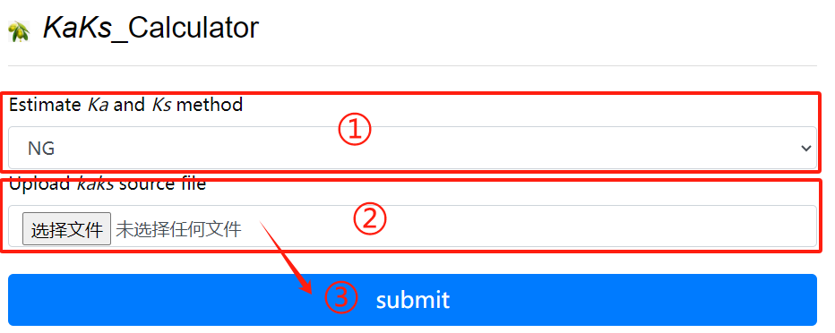
KaKs_Calculator usage:

1. Choose the method of estimate ka and ks
2. Upload kaks source file
3. Click the submit button

Hmmer

Reference: HMMER: biosequence analysis using profile hidden Markov models

Download: hmmer-3.3.tar.gz ↗ [Source]

Online address. http://www.ebi.ac.uk/Tools/hmmer/
Local download address. http://hmmer.org/

Use Flow:

## HMMER is a very powerful software package for biological sequence analysis work based on Hidden Markov Model, its general use is to identify homologous protein or nucleotide sequences and perform sequence comparison. Compared to sequence alignment and database search tools such as BLAST and FASTA, HMMER is more accurate.
1. Usage
HMMER can be accessed online or as a command line tool for local download and installation.

# hmmbuild [-options]

# The input file msafile is the file after multiple sequence alignment and supports many biological data formats such as: CLUSTALW, SELEX, GCG MSF.
# hmmbuild can automatically determine the type of input sequences (nucleic acid or protein), and the user can specify the type of input sequences as follows
    --amino: protein comparison sequence
    --dna: DNA alignment sequence
    --rna: RNA alignment sequence
# The output file hmmfile_out is generally named with .hmm suffix, the result of the HMM database, the user does not get much readable information.

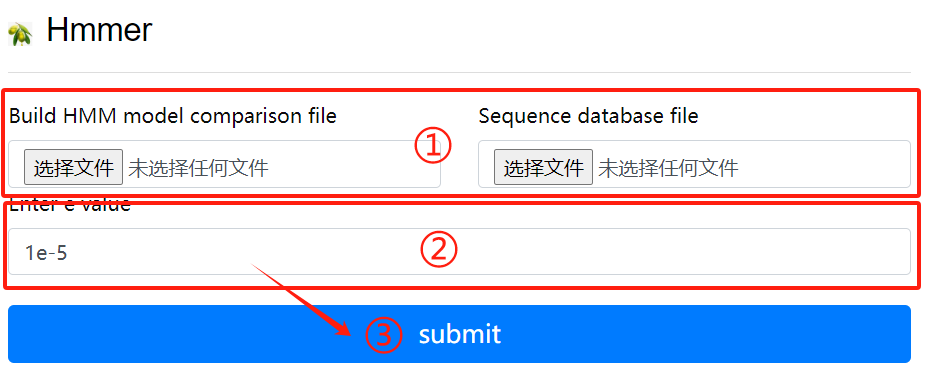
Hmmer usage:

1. Upload hmm file to create HMM comparison
   model
2. Upload purpose fasta file
3. Click the submit button

Pfam

Reference: Pfam: the protein families database

Download: Pfam-A.hmm.gz ↗ [Source]

 Pfam-A.hmm.dat.gz 
 Pfam-A.seed.gz 
 Pfam-A.full.gz 
Formatting the Pfam database via hmmerspress

Use Flow:

Run the program
    nohup pfam_scan.pl -fasta /your_path/masp.protein.fasta -dir /your_path/PfamScan/Pfam_data -outfile masp_pfam -cpu 16 &

# The results of the analysis of the structural domain part of the pfamscan protein are described below:
    (1) seq_id: transcript ID+[0,1,2], transcripts that do not exist in the list are noncoding
    (2) hmm start: the starting position of the domain compared to the structure
    (3) hmm end: compare to the end position of the structural domain
    (4) hmm acc: ID of the pfam domain
    (5) hmm name: the name of the pfam structured domain
    (6) hmm length: the length of the pfam structured domain
    (7) bit score: the score of the pair
    (8) E-value: the E-value of the comparison, the pfam structure domain filtering condition is: Evalue < 0.001

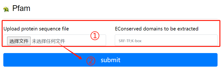
Pfam usage:

1. Upload purpose fasta file and select the
   destination domain
2. Click the submit button

MEME

Reference: MEME SUITE: tools for motif discovery and searching

Download: meme-5.5.4.tar.gz ↗ [Source]

Installation:

# The latest version of MEME relies on perl version 5.10.1 and above, so perl needs to be installed. Download perl and install it.
#
    tar zxvf perl.tar.gz
    cd /yourpath/perl
    . /Configure -des -Dprefix= /yourpath/perl_Dusethreads
    make ##take a lot of time
    make test
    make install
    .bash_profile #Write your installation path

    tar zxf meme.tar.gz
    cd meme_4.11.3
    ./configure --prefix=/yourpath/meme --with-url=http://meme-suite.org --enable-build-libxml2 --enable-build-libxslt
    make
    make test
    make install

MEME Official download page.
Download Releases - MEME Suite (meme-suite.org)

Use Flow:

The following is referenced in the MEME Manual (http://meme-suite.org/doc/overview.html?man_type=web)

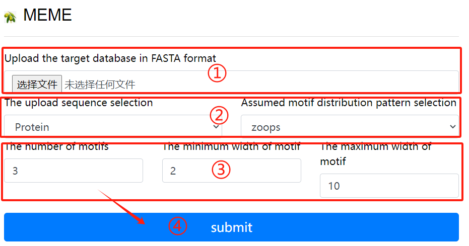
MEME usage:

1. Upload the target fasta sequence
2. Select the sequence format to upload and
   Select a hypothetical motif distribution
   pattern
3. Select the required parameters
4. Click the submit button

CpgFinder

Reference: CPG Island Finder with Sliding Window Algorithm: String Index Out of Bound Exception intermittently

Download: ↗ [Source]

Use Flow:

The program is intended to search for CpG islands in sequences.

Program options:
Min length of island to find - searching CpG islands with a length (bp) not less than specified in the field.
Min percent G and C - searching CpG islands with a composition not less than specified in the field.
Min CpG number - the minimal number of CpG dinucleotides in the island.
Min gc_ratio=P(CpG)/(expected)P(CpG) - the minimal ratio of the observed to expected frequency of CpG dinucleotide in the island.
Extend island if its lengths less then required - extending the CpG island, if its length is shorter than required.

Output example:

Search parameters:  len: 200   %GC: 50.0   CpG number: 0   P(CpG)/exp: 0.600   extend island: no   A: 21   B: -2
Locus name:  9003..16734 note="CpG_island (%GC=65.4, o/e=0.70, #CpGs=577)"
Locus reference:   expected P(CpG): 0.086   length: 25020
    20.1%(a)  29.9%(c)  28.6%(g)  21.4%(t)   0.0%(other)

				FOUND 4 ISLANDS
  #     start      end   chain   CpG    %CG    CG/GC    P(CpG)/exp     P(CpG)    len
  1      9192    10496     +     161   73.0    0.847   0.927( 1.44)    0.123    1305
  2     11147    11939     +      87   69.2    0.821   0.917( 1.28)    0.110     793
  3     15957    16374     +      57   79.4    0.781   0.871( 1.60)    0.137     418
  4     14689    15091     +      49   74.2    0.817   0.887( 1.42)    0.122     403

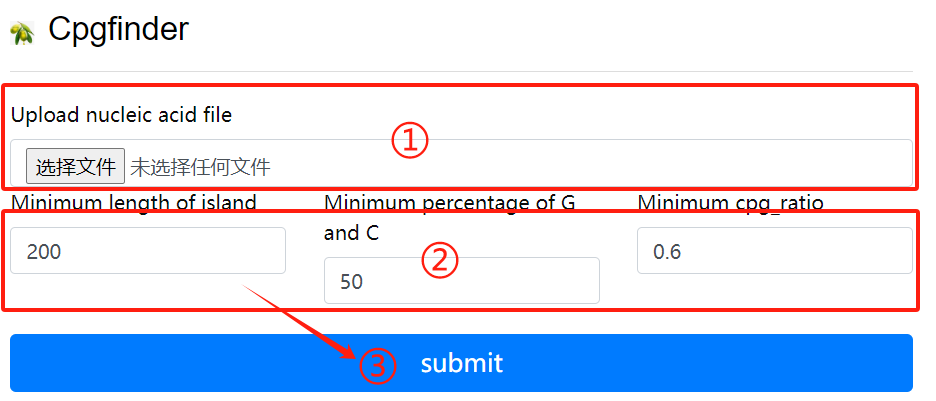
CpgFinder usage:

1. Upload nucleic acid file
2. Select the required parameters
3. Click the submit button

Codonw

Reference: Codon Pattern of Papillomavirus (Type I) from Bos Grunniens Based on the CodonW Software

Download: CodonWSourceCode_1_4_4.zip ↗ [Source]

Installation:

# Linux version.
# Install directly with conda, just type the command.
    conda install codonw
    codonw
        Welcome to CodonW  for Help type h
     Initial Menu
    Option
    (1) Load sequence file
    ( )
    (3) Change defaults
    (4) Codon usage indices
    (5) Correspondence analysis
    ( )
    (7) Teach yourself codon usage
    (8) Change the output written to file
    (9) About C-codons
    (R) Run C-codons
    (Q) Quit
    Select a menu choice, (Q)uit or (H)elp ->

Use Flow:

    Codon usage indices
    Options
    ( 1) {Codon Adaptation Index       (CAI)           }
    ( 2) {Frequency of OPtimal codons  (Fop)           }
    ( 3) {Codon bias index             (CBI)           }
    ( 4) {Effective Number of Codons   (ENc)           }
    ( 5) {GC content of gene           (G+C)           }
    ( 6) {GC of silent 3rd codon posit.(GC3s)          }
    ( 7) {Silent base composition                      }
    ( 8) {Number of synonymous codons  (L_sym)         }
    ( 9) {Total number of amino acids  (L_aa )         }
    (10) {Hydrophobicity of protein    (Hydro)         }
    (11) {Aromaticity of protein       (Aromo)         }
    (12)  Select all
    (X)  Return to previous menu
    Choices enclosed with curly brackets are the current selections
    Select a menu choice, (Q)uit or (H)elp ->

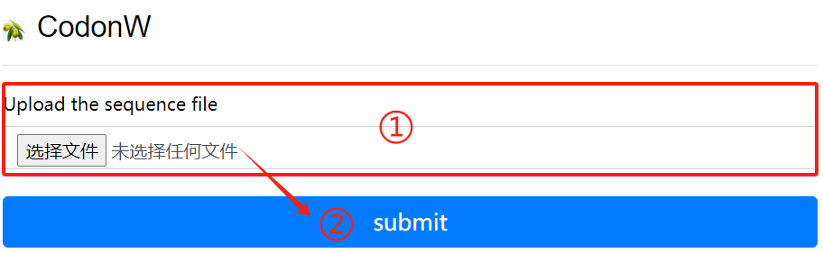
CodonW usage:

1. Upload the sequence file
2. Click the submit button

IQ-Tree

Reference: IQ-TREE: a fast and effective stochastic algorithm for estimating maximum-likelihood phylogenies

Installation: ↗ [Source]

conda install iqtree

Use Flow:

    iqtree -s example.phy -m MF -mtree -T AUTO
    iqtree -s example.phy -m GTR+I+G
    iqtree -s example.phy -m MFP -b 1000 -T AUTO
    iqtree -s example.phy -m MFP -B 1000 --bnni -T AUTO

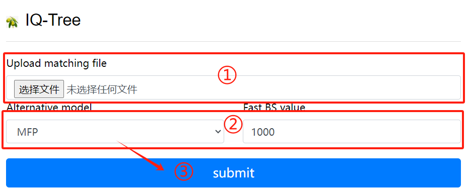
IQ-Tree usage:

1. Upload matching file
2. Select alternative models and BS values
3. Click the submit button

FastTree

Reference: FastTree: computing large minimum evolution trees with profiles instead of a distance matrix

Download: FastTree ↗ [Source]

Installation:

conda install fasttree

Use Flow:

fasttree -nt nucleotide_alignment_file > tree_file
fasttree protein_alignment_file  tree_file

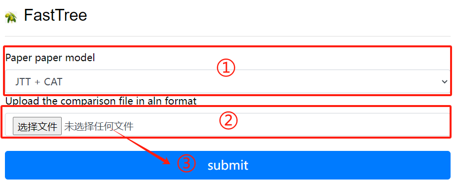
FastTree usage:

1. Selective calculation model
2. Upload the comparison file in aln format
3. Click the submit button

SequenceServer

Reference: Sequenceserver: A Modern Graphical User Interface for Custom BLAST Databases

Installation: ↗ [Source]

    sudo apt-get install ruby gem ruby-dev
    sudo gem install sequenceserver
    scp /dbindex usr@ip:/home/db
    sequenceserver -m -d /db

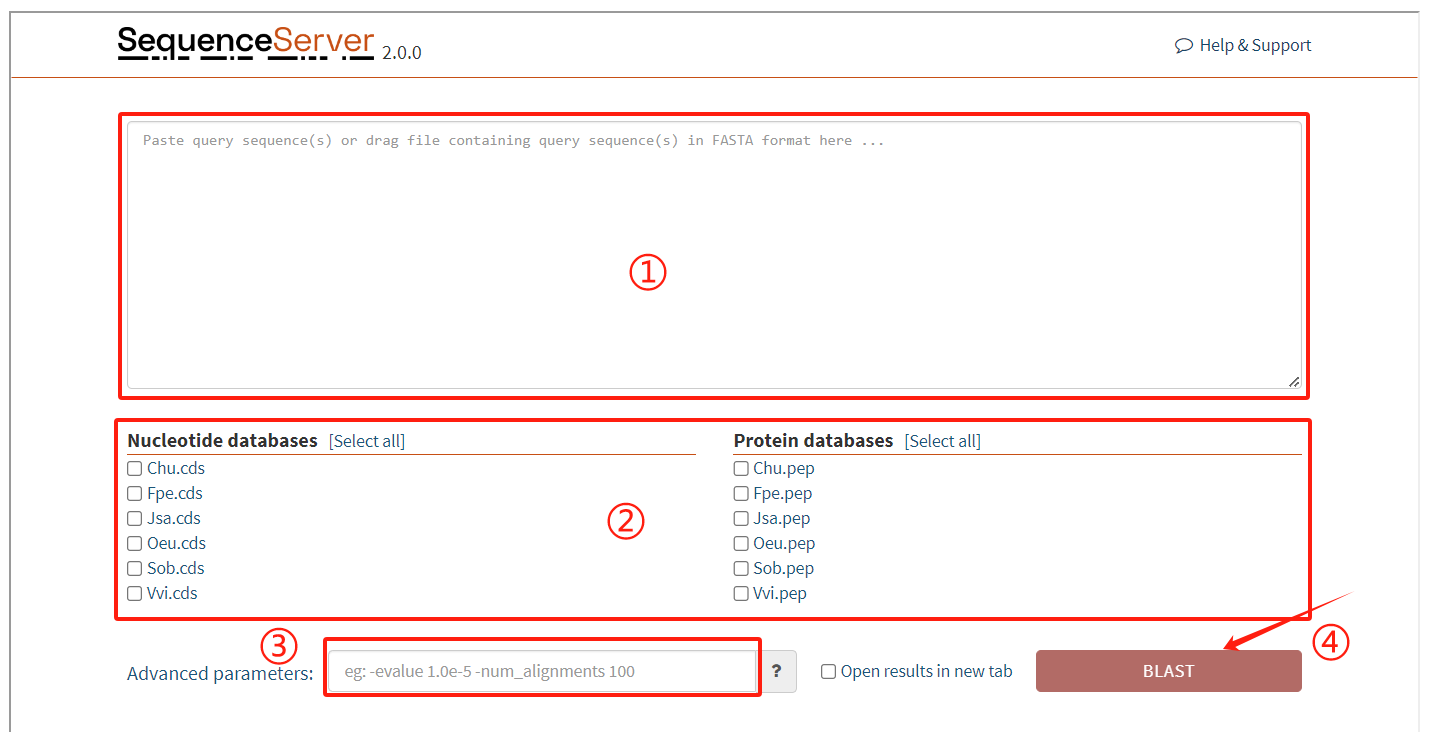
SequenceServer usage:

1. Enter the target sequence to be matched
2. Select the corresponding database
3. Enter the required parameters
4. Click the submit button

Synvisio

Use Flow:

    Synvisio is an interactive multiscale visualization tool that allows you to explore the results of McScanX. We have created a complete genome library of species on the server, where users can select species for synteny analysis and display detailed synteny relationships between different chromosomes.

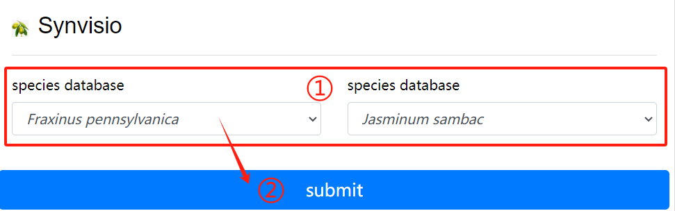
Synvisio usage:

1. Choose to want to see the two species of
   genome database
2. Click the submit button

NG_KaKs_Cal

Download: run_ks.py

Use Flow:

    KaKs represents the ratio between the non synonymous substitution rate (Ka) and synonymous substitution rate (Ks) of two protein coding genes. This ratio can determine whether there is selective pressure on the protein coding gene. Upload block file and CDS file.

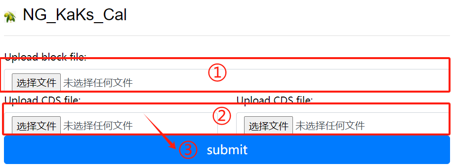
NG_KaKs_Cal usage:

1. Upload block file
2. Upload corresponding cds file
3. Click the submit button

BBK_Dotter

Download: run_ks_dot.py

Use Flow:

    BBK_Dotter is a genome structure lattice diagram drawn based on the results of blast sequence alignment and block synteny, with Ks values labeled next to the block. Upload BLAST file, block file, Ks file, species lens file and species gff file.

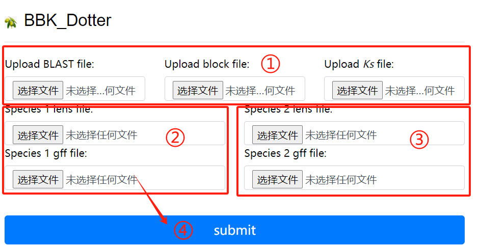
BBK_Dotter usage:

1. Upload the blast block ks file
2. Upload lens and gff corresponding to the
   first genome
3. Upload lens and gff corresponding to the
   second genome
4. Click the submit button

GSDS

Reference: GSDS 2.0: an upgraded gene feature visualization server

Download: gsds_v2.tar.gz ↗ [Source]

Installation:

a. Change to the path for installing GSDS 2.0 and unpack the tar package.
    cd $PATH2INSTALL_GSDS
	tar -zxvf gsds_v2.tar.gz
b. Modify the authetification of task directories and log file
    cd $PATH2INSTALL_GSDS/gsds_v2
	mkdir task, task/upload_file
	chmod 777 task/
	chmod 777 task/upload_file/
	chmod a+w gsds_log
c. Link CGI commands in directory gcgi_bin to the commands in your system
    cd $PATH2INSTALL_GSDS/gsds_v2/gcgi_bin
	ln -s -f seqretsplit
	ln -s -f est2genome
	ln -s -f bedtools
	ln -s -f rsvg-convert
d. Configure Apache2 for accessing GSDS 2.0

Seq alignment

Use Flow:

    Multiple sequence alignment tool selection, including mafft, muscle and clustalw2.

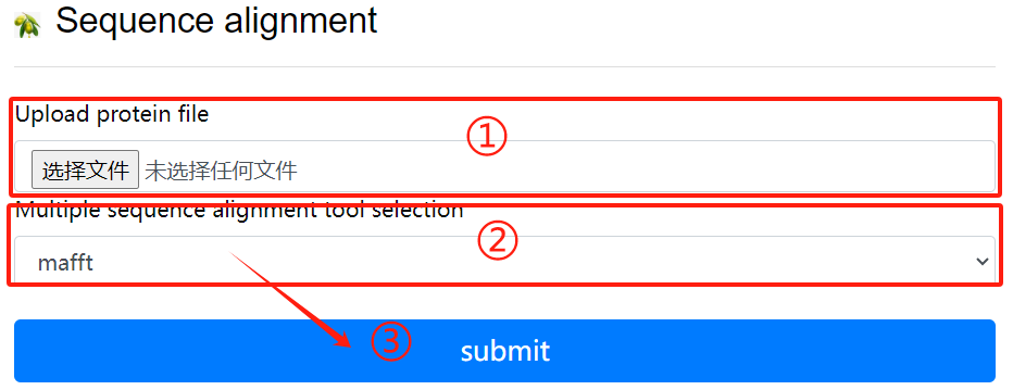
Seq alignment usage:

1. Upload protein file
2. Multiple sequence alignment tool
   selection
3. Click the submit button

Phyml

Reference: New algorithms and methods to estimate maximum-likelihood phylogenies: assessing the performance of PhyML 3.0

Download: PhyML-3.1.zip ↗ [Source]

Installation:

$ unzip PhyML-3.1.zip
$ mv PhyML-3.1 /opt/biosoft/
$ ln -s /opt/biosoft/PhyML-3.1/PhyML-3.1_linux64 /opt/biosoft/PhyML-3.1/PhyML
$ echo 'PATH=$PATH:/opt/biosoft/PhyML-3.1/' >> ~/.
$ source ~/.bashrc

Use Flow:

$ PhyML -i proteins.phy -d aa -b 1000 -m LG -f m -v e -a e -o tlr
    -i seq_file_name
    -d data_type default：nt
    -b int
    -m model
    -f e,m or fA,fC,fG,fT
    -v prop_invar
    -a gamma
    -o params

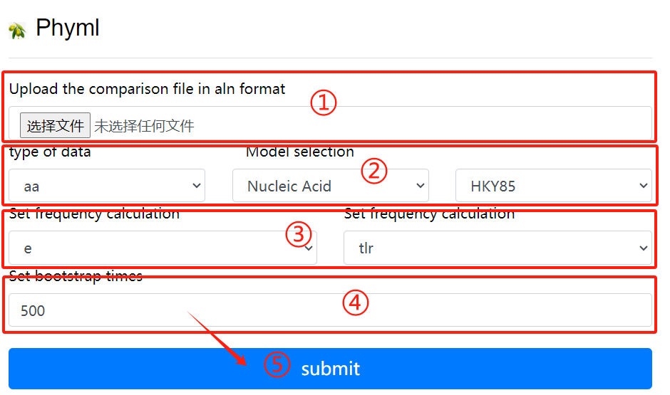
Phyml usage:

1. Upload the comparison file in aln format
2. Select the data type and model
3. Set frequency calculation
4. Set bootstrap times
5. Click the submit button

SS-extractor

Use Flow:

class sequence_run2(object):
    def __init__(self, place):
        self.id_list = []
        self.place = place

    def new_prot(self):
        new_prot = open(f'{path_get}/file_keep/{self.place}/new_pro.txt', 'w')
        for line in SeqIO.parse(f'{path_get}/file_keep/{self.place}/protein.fasta', 'fasta'):
            if line.id in self.id_list:
                new_prot.write('>' + str(line.id) + '\n' + str(line.seq) + '\n')

    def new_cds(self):
        new_cds = open(f'{path_get}/file_keep/{self.place}/new_cds.txt', 'w')
        for line in SeqIO.parse(f'{path_get}/file_keep/{self.place}/gene.fasta', 'fasta'):
            if line.id in self.id_list:
                new_cds.write('>' + str(line.id) + '\n' + str(line.seq) + '\n')

    def new_gff(self):
        new_gff = open(f'{path_get}/file_keep/{self.place}/new_gff.txt', 'w')
        gff_file = open(f'{path_get}/file_keep/{self.place}/gff.fasta', 'r')
        for line in gff_file:
            gff_id = line.split()[1]
            if gff_id in self.id_list:
                new_gff.write(line)

    def main(self):
        id_file = open(f'{path_get}/file_keep/{self.place}/id.fasta', 'r')
        for line in id_file.readlines():
            self.id_list.append(line.split()[0])
            self.new_prot()
            self.new_cds()
            self.new_gff()

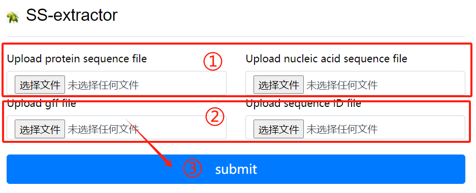
SS-extractor usage:

1. Upload protein sequence file and nucleic
   acid sequence file
2. Upload gff file and sequence id file
3. Click the submit button

SAF-converter

Use Flow:

def format_fasta_run(place, file_name, patten, patten_end, file_last):
    SeqIO.convert(f"{path_get}/file_keep/{place}/{file_name}.{file_last}", f"{patten}",
                  f"{path_get}/file_keep/{place}/{file_name}.{patten_end}", f"{patten_end}")

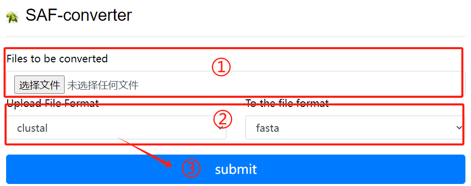
SAF-converter usage:

1. Upload the file to be converted
2. Select the file format to upload and the
   file format to convert
3. Click the submit button

BDI-deduplicator

Use Flow:

def quchong_run(place):
    id_list = []
    new_file = open(f'{path_get}/file_keep/{place}/new.fasta', 'w')
    for line in SeqIO.parse(f'{path_get}/file_keep/{place}/1.fasta', 'fasta'):
        if line.id not in id_list:
            id_list.append(line.id)
            new_file.write(">" + str(line.id) + "\n" + str(line.seq) + "\n")
    new_file.close()

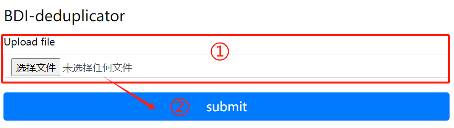
BDI-deduplicator usage:

1. Upload files that need to
   delete duplicate sequences
2. Click the submit button

BDI-extractor

Use Flow:

def extr_row_run(place, row_num, row_name, row_last):
    cmd = f"""
        cd {path_get}/file_keep/{place}
        cut -f {row_num} {row_name}.{row_last} > {row_name}.new.{row_last}
    """
    subprocess.run(cmd, shell=True, check=True)

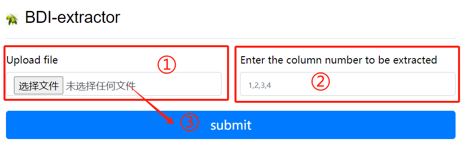
BDI-extractor usage:

1. Upload a gff file
2. Enter the column number to be extracted
3. Click the submit button

BDI-combiner

Use Flow:

def file_merge_run_tools(place):
    cmd = f"""
        cd '{path_get}/file_keep/{place}'
        cat orthomcl/* >> result.txt
    """
    subprocess.run(cmd, shell=True, check=True)

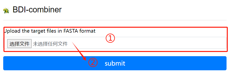
BDI-combiner usage:

1. Upload files
2. Click the submit button

ShinyCircos

Reference: shinyCircos: an R/Shiny application for interactive creation of Circos plot

Download: shinyCircos-master.zip ↗ [Source]

Installation:

install.packages("shiny")
install.packages("circlize")
install.packages("RColorBrewer")
install.packages("data.table")
install.packages("RLumShiny")
## try http:// if https:// URLs are not supported
source("https://bioconductor.org/biocLite.R")
biocLite("GenomicRanges")

Use Flow:

# Define the user to spawn R Shiny processes
run_as shiny;

# Define a top-level server which will listen on a port
server {
  # Use port 3838
  listen 3838;
  # Define the location available at the base URL
  location /shinycircos {
    # Directory containing the code and data of shinyCircos
    app_dir /srv/shiny-server/shinyCircos;
    # Directory to store the log files
    log_dir /var/log/shiny-server;
  }
}

Syn_Ks_Dis

Download: new-ksdistribution.V3.R

Use Flow:

Rscript new-ksdistribution.V3.R ks_input.csv ksargs.png 6 5 300

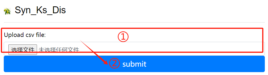
Syn_Ks_Dis usage:

1. Upload csv file
2. Click the submit button

B_Dotter

Download: dotplot.pl

Use Flow:

perl dotplot.pl

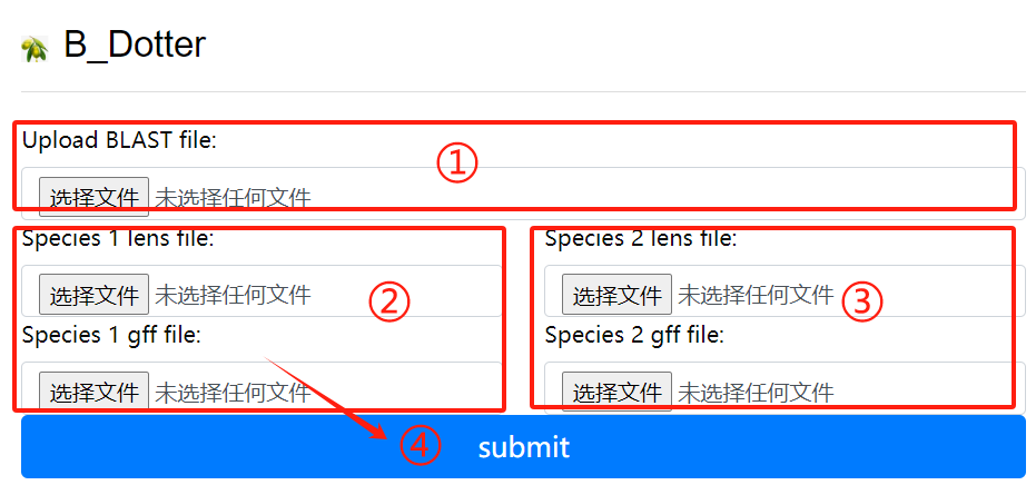
B_Dotter usage:

1. Upload the blast file
2. Species 1 lens file and 1 gff file
3. Species 2 lens file and 2 gff file
4. Click the submit button

BB_Dotter

Download: dotplot_block.2400.pd.py

Use Flow:

python dotplot_block.2400.pd.py

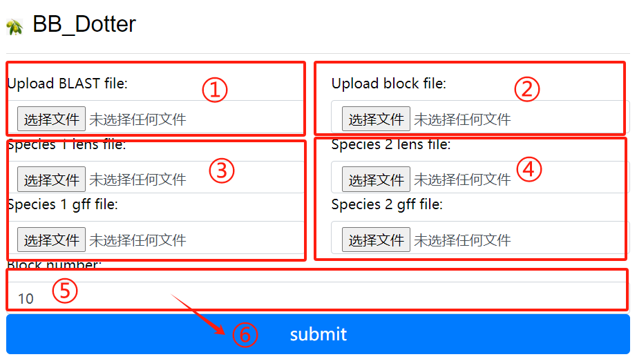
BB_Dotter usage:

1. Upload the blast file
2. Upload the block file
3. Species 1 lens file and 1 gff file
4. Species 2 lens file and 2 gff file
5. Upload block number
6. Click the submit button

Paleo-gene_identifer

Download: corr_dotplot_spc_last.py

Use Flow:

python corr_dotplot_spc_last.py

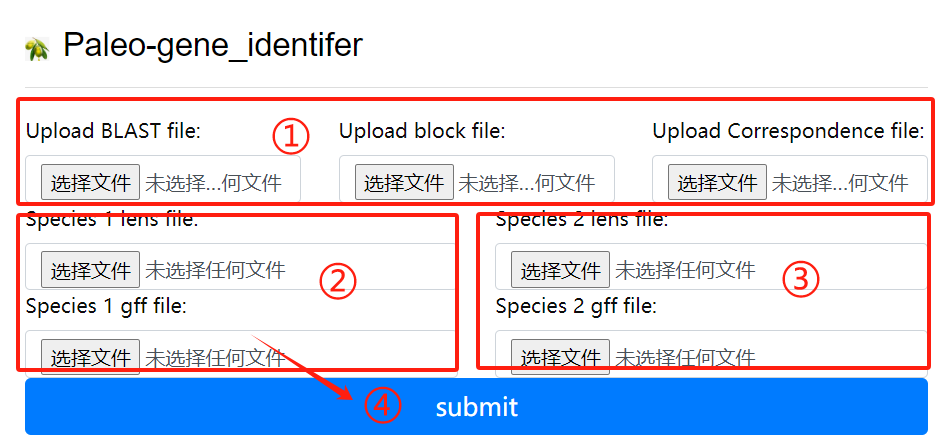
Paleo-gene_identifer usage:

1. Upload the blast block and
   correspondence file
2. Species 1 lens file and 1 gff file
3. Species 2 lens file and 2 gff file
4. Click the submit button

Paleo-gene_RI

Download: baoliu.py

Use Flow:

python baoliu.py

Paleo-gene_RI usage:

1. Upload the mc file
2. Click the submit button

Paleo-gene_RII

Download: lost.py

Use Flow:

python lost.py

Paleo-gene_RII usage:

1. Upload the mc file
2. Click the submit button

WGDI

Reference: WGDI: A user-friendly toolkit for evolutionary analyses of whole-genome duplications and ancestral karyotypes

Download: ↗ [Source]

Use Flow:

## More details on the steps or process of using WGDI can be found. https://wgdi.readthedocs.io/en/latest/Introduction.html

Dupgen finder

Reference: Gene duplication and evolution in recurring polyploidization-diploidization cycles in plants

Download: DupGen_finder-master.zip ↗ [Source]

Installation:

cd DupGen_finder
make
chmod 775 DupGen_finder.pl
chmod 775 DupGen_finder-unique.pl
chmod 775 set_PATH.sh
source set_PATH.sh

Use Flow:

# geneDuplication analysis
# The geneDuplication analysis, using DupGen-finder, can classify all genes into 5 categories according to their replication types
    WGD: whole genome duplication
    TD: Tandem duplication (two duplicated genes next to each other)
    PD: proximal duplication (duplicated genes within 10 genes apart)
    TRD: Transpositional duplication (duplicated genes consisting of an ancestor and a new locus)
    DSD: scattered duplication (duplicated genes that are not adjacent nor coterminous)
    SL: single copy
# require input file

# analysis of mode 1 (comparison with itself) and mode 2 (comparison with other species)
# analyze mode 1
    cat Spd.bed |sed 's/^/Spd-/g'|awk '{print $1"\t"$4"\t"$2"\t"$3}' >Spd.gff
    cat Ath.bed |sed 's/^/Ath-Chr/g'|awk '{print $1"\t"$4"\t"$2"\t"$3}' >Ath.gff
    sed -i 's/Chr0/Chr/g' Spd.gff

    cat Spd.gff Ath.gff >Spd_Ath.gff

    makeblastdb -in Spd.pep -dbtype prot -title Spd -parse_seqids -out Spd
    blastp -query Spd.pep -db Spd -evalue 1e-10 -max_target_seqs 5 -outfmt 6 -out Spd.blast
# Create a reference database
    makeblastdb -in Ath.pep -dbtype prot -title Ath -parse_seqids -out Ath
# Align protein query sequences against the reference database
    blastp -query Ath.pep -db Ath -evalue 1e-10 -max_target_seqs 5 -outfmt 6 -out Ath.blast
    mkdir Spd_Ath
    cat Spd.blast Ath.blast >Spd_Ath.blast

# -t is the experimental group -c is the exogenous control group
# General mode
    DupGen_finder.pl -i $PWD -t Spd -c Ath -o ${PWD}/Spd_Ath/results1
# Strict mode
    DupGen_finder-unique.pl -i $PWD -t Spd -c Ath -o ${PWD}/Spd_Ath/results2

GF_circos

Download: Excircle.zip

Use Flow:

GF_circos is a tool for analyzing chromosomal localization and expansion patterns of family genes.
The installation package contains instances, prepare files based on the examples, and conf is the
configuration file. Fill in the corresponding data file.

Command:    python .\run.py excircle -c excircle.conf

Transcriptome analysis

Download: ↗ [Trimmomatic] ↗ [SRA-Toolkit] ↗ [fastqc] ↗ [hisat2] ↗ [samtools] ↗ [stringtie]

I: Convert SRA data to fastq format using fasterq-dump
# fasterq-dump --split-3 *.sra
II: Use fastQC to evaluate the quality of fastq files
# fastqc *fq
III: The splices are removed, the bases are pruned, and low quality sequences are filtered.
# trimmomatic PE -threads 4 -phred33 *_1.fastq.gz *_2.fastq.gz *_1_clean.fq *_1_unpaired.fq *_2_clean.fq *_2_unpaired.fq
  ILLUMINACLIP:TruSeq3-PE.fa:2:30:10 LEADING:20 TRAILING:20 SLIDINGWINDOW:4:20 MINLEN:50 (Double-ended sequencing)
  trimmomatic SE -threads 4 -phred33 *.fastq.gz *_clean.fq
  ILLUMINACLIP:TruSeq3-SE.fa:2:30:10 LEADING:20 TRAILING:20 SLIDINGWINDOW:4:20 MINLEN:50 (Single-ended sequencing)
IV: Build an index of the reference genome
# hisat2-build -p 3 *.fa *.index
V: The fasta sequences were aligned to the reference genome
# hisat2 --new-summary --rna-strandness RF -p 10 -x *.index -1 *_1_clean.fq -2 *_2_clean.fq -S *.sam (Double-ended sequencing)
# hisat2 --new-summary --rna-strandness R -p 10 -x *.index -U *_clean.fq -S *.sam (Single-ended sequencing)
VI: Conversion of bam and sam
# samtools sort -o *.bam *.sam
VII: Quantitative analysis of gene expression
# stringtie -e -A *.out -p 4 -G *.gtf -o *.gtf *.bam

iTAK

Reference: iTAK: a program for genome-wide prediction and classification of plant transcription factors, transcriptional regulators, and protein kinases.

Download: iTAK ↗ [Source]

Use Flow:

Use of the online version
    1. Input the data and select the data type. Protein sequence data can be uploaded in file form or directly pasted in FASTA format sequence.
    2. Fill in the email address for receiving data.
Result interpretation
    tf_sequence.fasta
    All identified TF/TR sequences

    tf_classification.txt
    The classification of all TF/TR, tab TAB character segmentation, including the ID of the sequence and their respective families.

    tf_alignment.txt
    A table-segmented txt document, containing a database of all identified TF/TR alignment protein domains.

    pk_sequence.fasta
    All the identified PK protein sequences.

    Shiu_classification.txt
    Classification of all identified PK proteins. A table-segmented txt file containing sequence ID and the corresponding protein kinase family.

    Shiu_alignment.txt
    A table-segmented txt document, containing a database of all identified PK comparison protein domains.


Download and install
    conda install -c bioconda itak

Usage
    iTAK.py sequence_file

Interproscan

Download: Interproscan ↗ [Source]

Use Flow:

Download and install
    wget https://ftp.ebi.ac.uk/pub/software/unix/iprscan/5/5.61-93.0/interproscan-5.61-93.0-64-bit.tar.gz
    tar -pxvzf interproscan-5.61-93.0-*-bit.tar.gz
    cd interproscan-5.61-93.0
    export PATH=`pwd`:$PATH

* Note that the software relies on Java11 or above
    export PATH=/home/public/tools/jdk-17.0.1/bin:$PATH
Protein sequence
    interproscan.sh -cpu 40 -d anno.dir -dp -i protein.fa
Nucleic acid sequence
    interproscan.sh -cpu 40 -d anno.dir -dp -t n -i transcripts.fa

- Number of cpu threads
-d Output directory
-dp does not use existing calculation results (seems to require networking?)
-i Indicates the sequence of comments